
[논문리뷰] Masked Autoencoders Are Scalable Vision Learners
이번 포스팅에서는 2021년 11월 11일에 발표된 Masked Autoencoders Are Scalable Vision Learners 논문을 모델 구현과 함께 리뷰하려고 한다. 해당 논문은 FAIR(Facebook AI Research)의 Kaiming He가 1저자로 나온다. (Kaiming He라는 이름만으로 또 어떤 아이디어를 제시했을지 기대하게 되는것 같다.)
이 논문에서 제시한 Masked Autoencoder(이하 MAE)는 Self-Supervised Learning 분야를 다루는 모델이다. 논문을 다루기 전에 먼저 Self-Supervised Learning에 대해 알아보자
Self-Supervised Learning
딥러닝 분야에서 가장 많이 사용되는 Supervised Learning의 가장 큰 문제점은 데이터에 대한 정답(Label)이 구축되어야 한다는 것이다. Label을 구축하는데에는 분야에 따라 다르지만 대부분 많은 시간과 비용이 투자되어야 한다. 딥러닝 모델은 계속해서 발전해왔지만 이런 모델을 자신의 task에 적용하고 싶어도 데이터 구축에 많은 어려움이 있는것이 현실이다.
이러한 문제에서 벗어날 수 있는 방법으로는 Unsupervised Learning, Semi-Supervised Learning이 있지만 최근 Self-Supervised Learning이라는 연구 방법이 주목을 받고 있다. Self-Supervised Learning은 아래와 같은 과정을 따른다.
- Pretext task를 정의한다. (MAE의 task는 이미지의 마스킹된 영역을 원본 이미지와 같도록 generate 하는것.)
- 데이터 자체의 정보를 사용하여 그것을 supervision으로 삼아 Pretext task를 목표로 학습시킨다.
- 학습한 모델을 평가하기 위해 2에서 학습시킨 모델을 Downstream task(classification 등)에 가져와 weight를 freeze 시킨 후 transfer learning을 수행한다. (2번을 통해 얼마나 feature extraction이 잘 이루어 졌는지 판단)
최근 NLP분야에서 유명한 GPT, BERT가 바로 Self-Supervised Learning으로 이루어졌다. GPT는 다음 단어를 예측한다면 BERT는 중간에 있는 단어를 채운다는 차이점이 있지만 데이터의 일부를 제거하여 그것을 예측한다는 공통적인 self supervision을 가진다.
Vision 분야에서도 Self-Supervised Learning 연구가 계속 되어왔지만 유독 NLP에 반해 약한모습을 보여왔는데 오늘 소개해 드릴 논문에서 그 이유와 MAE라는 모델로 가능성을 보여준다.
1. Introduction
GPT, BERT와 같이 NLP에서는 masked autoencoding이 좋은 성능을 보여주는데 Vision은 그렇지 못했던 것에 대해 저자들은 다음과 같이 정리하였다.
1. language와 vision의 architectural gap
- NLP와 달리 Vision에서는 일정 grid로 나뉘어 지역적으로 작동하는 CNN이 지배적이기 때문에 mask token이나 positional embedding을 활용하기 어렵다.
- 최근 VIT(Vision Transformer)가 나오게 되면서 이 문제가 극복되었다.
2. Information density is different between language and vision.
- 사람이 만든 언어는 단어 하나하나의 의미가 중요하고 정교한 language understanding이 학습되어 중간에 빠진 단어를 예측을 하는 방식이라면 이미지는 그냥 natural signal이고 spatial redundancy하기 때문에 주변 픽셀로 부터 어렵지 않게 정보를 얻어 비어있는 픽셀을 예측할 수 있다.
3. decoder 부분에서 language와 vision의 역할이 다르다.
- Vision에서는 decoder에서 reconstruct될 때 픽셀값이라는 low semantic information을 가지는 반면에 language에서 reconstruct 되는 단어는 rich semantic information을 가진다.
- decoder는 latent representation으로부터 semantic level을 결정하는 중요한 역할을 하기 때문에 low semantic information을 가지는 Vision에서는 decoder design이 잘 이루어져야 한다.
2. Related Work
Masked language modeling
- GPT, BERT와 같은 모델은 input sequence의 일부를 제거하고 pre-training해서 그 빈 공간을 예측하는 방식으로 좋은 성과를 내었다.
- 큰 모델로 pre-trained representation하여 일반화가 잘되고 다양한 downstream task에 적용할 수 있는 확장성을 갖추었다.
Autoencoding
- Autoencoder에서 encoder는 latent space로 매핑을 하고 decoder는 다시 input space로 reconstruct한다.
- 많이 사용하는 방법중 하나인 DAE(Denoising autoencoder)는 input signal에 노이즈를 추가하고 노이즈를 없애는 형태로 reconstruct하는 방식이다.
- masking pixels, removing color channel과 같은 방법을 생각해 볼 수 있음
Masked image encoding
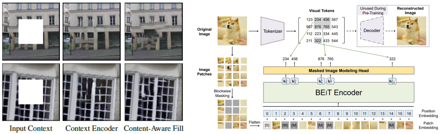
- DAE 이후에 이미지의 큰 마스킹된 영역을 CNN을 사용하여 채우는 Context Encoder
- NLP의 Transformer를 이미지 분류에 활용해 CNN과 견줄만한 성능을 보인 ViT
- 그리고 2021년 6월에 발표된 BEiT(BERT Pre-Training of Image Transformers)는 Transformer를 Self-Supervised Learning에 적용하였다.
3. Approach
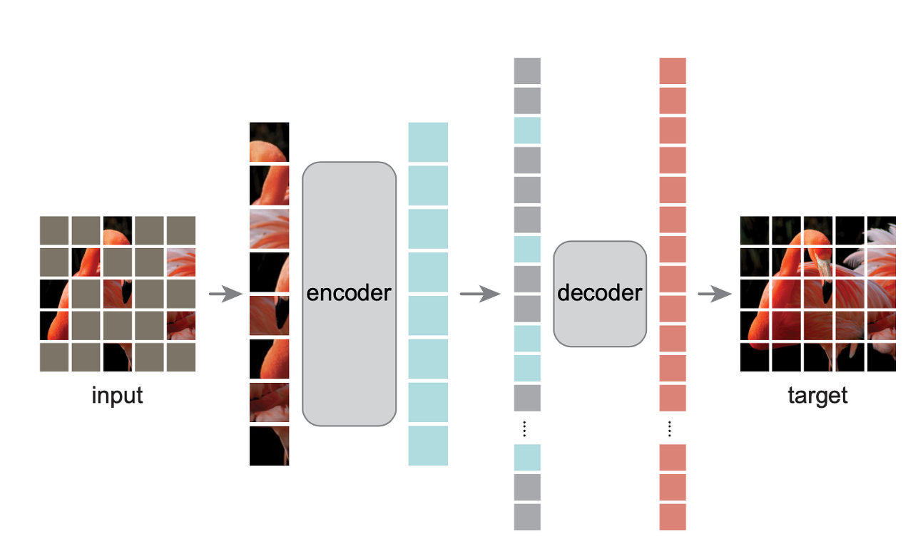
MAE는 기본적으로 Autoencoder의 컨셉을 따라간다. input signal을 latent representation시키고 다시 original signal로 reconstruct시킨다. 다만 기존의 Autoencoder와 다른점은 asymmetric design으로 구성했는데 encoder에는 masking 되지 않은 토큰만 사용하고 decoder에서는 encoder보다 조금 더 가볍에 모델링 함과 동시에 mask token을 붙여서 reconstruct시킨다.
Masking
- 먼저 Input은 ViT와 동일하게 nxn크기의 패치로 나눈다. 그리고 패치별로 랜덤하게 마스킹을 하게 되는데 이때 저자들은 uniform distribution으로 마스크를 random sampling하였다.
- 위 그림에서 볼 수있듯이 상당히 많은 패치를 마스킹하는 것을 볼 수 있는데 저자들은 중복을 없앰으로서 주변 패치를 활용해서 쉽게 문제를 해결할 수 없도록 유도하려고 했고 uniform distribution을 통해 마스킹 되지 않은 부분이 어느 한곳에 편향되지 않도록 하였다.
MAE encoder
- MAE encoder는 ViT의 encoder와 동일한 구조를 가진다.
- 하지만 MAE encoder는 unmasked patch만 input으로 활용한다는데에 ViT와 차이점을 둔다. 논문에서는 masked patch의 비율을 전체 patch의 75%로 default값을 정했고 결국 encoder에 들어가는 패치는 25%만 포함된다.
- 먼저 unmasked patch들을 linear projection(transformer를 사용하기 때문) 시키고 positional embedding(패치의 위치 파악용도)을 더해준뒤 encoding을 수행한다. (ViT의 class token은 사용하지 않음)
- 25%의 패치만 사용함으로써 일부의 연산과 적은 메모리만으로 매우 큰 encoder를 학습할 수 있게된다.
MAE decoder
- decoder에서는 encoder에서 나온 visible patch와 mask token을 둘 다 사용한다.
- decoding을 수행하기 전 mask token을 원래 자리에 넣어야 하기 때문에 여기서 mask token에 positional embedding을 더해준다.
- MAE decoder는 pre-training에서만 사용되고 downstream(recognition)에서 평가할때는 사용하지 않는다. 그렇기 때문에 decoder architecture는 encoder와는 독립적으로 유연하게 디자인할 수 있게 된다.
- 본 논문에서는 decoder가 encoder 연산량의 10%만 차지하도록 구성하였고 이것으로 pre-training time을 줄일 수 있었다고 한다.
Reconstruction target
- MAE 는 masked patch의 픽셀값을 예측하는것으로 reconstruct된다.
- MAE는 loss function으로 원본 이미지와 픽셀값의 차이를 쉽게 구할 수 있는 MSE(Mean Square Error)를 사용하였다.
- 이때 오직 masked patch 영역에 대해서만 loss를 계산하게 된다.
- 각각의 patch에 대해서 normalization하여 resonstruction target을 normalized pixel로 뽑도록 하면 representation quality가 향상된다고 한다.
Simple implementation
- 먼저 이미지를 서로 겹치지 않는 패치로 나눈 다음에 linear projection + positional embedding을 적용한다.
- token을 random shuffle하여 masking ratio(75%)만큼 패치를 masking한다.
- unmasked patch만 인덱싱하여 encoding을 수행한다.
- encoded patch들과 mask token을 다시 list up하고 원래 위치로 unshuffle한다. (positional embedding 추가)
4. ImageNet Experiments
논문에서 self-supervised pre-training에 ImageNet-1K dataset을 사용하였다. 그 후 모델의 representation을 평가하기 위해 supervised learning을 수행할때 1) end-to-end fine-tuning 방법과 2) linear probing 방법 두가지를 사용했다.
Baseline으로는 VIT-Large 모델을 택했는데 이 모델은 굉장히 크고 overfit되는 경향이 있다. ViT-L, strong regularization을 추가한 ViT-L, fine tuning을 사용한 MAE와의 supervised 결과에 대한 비교는 다음과 같다.
4.1. Main Properties
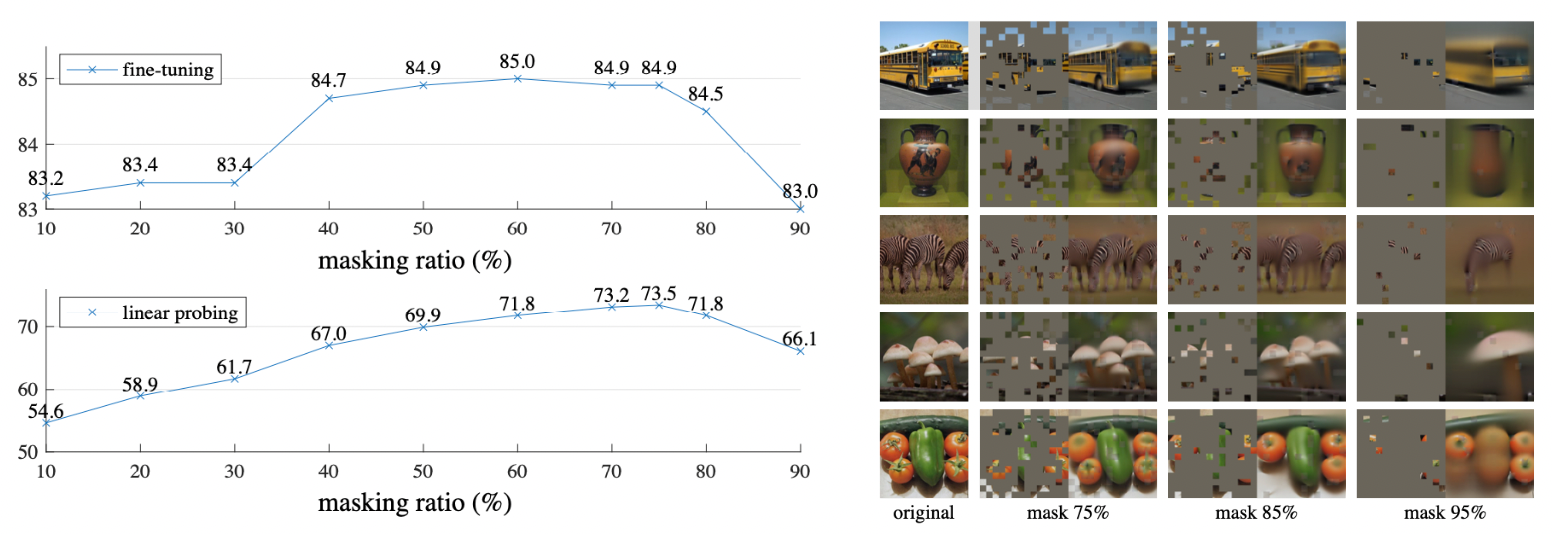
Masking ratio
- finetuning, linear probing방법 모두 75% masking에서 제일 높은 성능을 보였다.
- BERT에서는 15%만 masking하였지만 MAE는 75%나 마스킹을 했는데에도 불구하고 좋은 performance를 보이고 있다. 물론 task가 다르긴 하지만 같은 task에서 지금까지 나온 모델들도 20%~50%밖에 마스킹을 하지 못했다.
- 위 사진을 보면 원본 이미지에 비해 약간 blury하지만 꽤 그럴듯한 output을 생성해낸다. 이것은 단순히 선이나 질감을 넘어서 물체와 장면의 형태를 이해한다고 볼 수 있다.
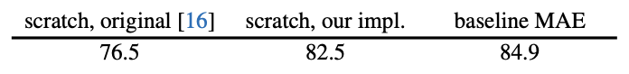
- linear probing과 fine tuning과의 accuracy gap이 굉장의 유의하고 fine-tuning은 어떠한 masking ratio에서도 저자들이 implement한 ViT scratch의 성능보다 높다.(82.5%)
Decoder design
Decoder는 downstream에서 사용하지 않는다는 것을 기억하고 이해하면 도움이 된다.
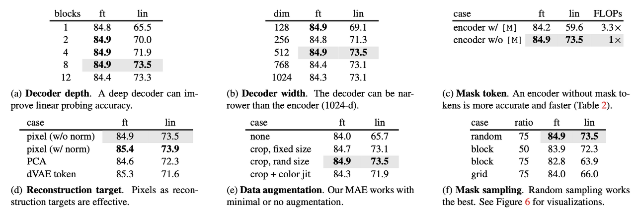
- 위 테이블(a), (b)에서 보이는 것과 같이 MAE의 decoder는 flexibly design되었다.
- decoder depth에서 fine tuning은 block이 한개만 있어도 성능이 최고치를 달성하지만 linear probing은 block의 개수에 따라 linear하게 성능이 올라간다. 특히 linear probing의 결과에 대해 저자들은 encoder 뒤의 마지막 몇 레이어는 reconstruction을 위해 더 specialized되지만 image recognition에서는 관련성이 덜하기 때문에 많은 레이어가 필요하다고 한다.
- 하지만 fine-tuning같은 경우에는 encoder의 마지막 layer를 조정하여 image recognition에 적응하기 때문에 block이 1개 이상 있으면 성능에 크게 영향을 주지 않는다. 즉 block수를 줄여 small decoder로 training이 가능하다.
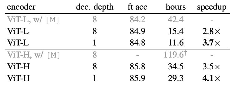
- 아래와 같이 fine-tuning에서는 depth에 따라 accuracy 차이가 미미하지만 학습 시간을 많이 단축할 수 있다.
Mask token
- 앞서 나온대로 MAE에서는 encoder에서 mask token을 사용하지 않고 decoder에 들어가기 전에 mask token을 ecoded patch에 붙이게 된다.
- table(c)에 보이는것과 같이 encoder에 mask token을 붙이지 않았을때 accuracy를 높이면서 3.3x FLOPs를 줄일 수있게 된다.
- 특히 linear probing에서 mask token을 encoder에 사용했을때 59.6%라는 낮은 accuracy가 나오는 이유는 pre-training과 deploying과의 gap이 있기 때문이다. pre-training에서 mask token을 사용하지만 결국 deploying에서는 visible 패치만 들어가버리는 gap이 생기기 때문에 deploying 단계에서 성능저하가 일어난다.
Reconstruction target
- MAE에서는 patch별로 pixel값을 normalization함으로써 성능을 향상시켰다.
- PCA, dVAE(토큰을 예측하기 위해 한번 더 pre-training 필요)와 같은 방법들을 시도해보았지만 여러 방면에서 pixel normalization이 가장 경쟁력이 있다. (테이블(d) 참고)
Data augmentation
- Image augmentation 기법들은 수도없이 많지만 MAE에서는 단순히 radom horizontal flip, cropping만 사용하였다.
- 심지어 단순히 center-crop만 사용해도 잘 작동이 된다고 하는데 그 이유는 바로 ramdom masking이 augmentation역할을 하기 때문이라고 한다. each iteration마다 다른 mask를 취하기 때문에 data augmentation없이 새로운 학습데이터가 생성되는 것이다.
- 이런 마스킹 작업을 통해 Pretext task를 더 어렵게 만들어주고 train regularize를 위해서 적은 augmentaion이 필요하다고 한다. (테이블(e) 참고)
Mask sampling strategy
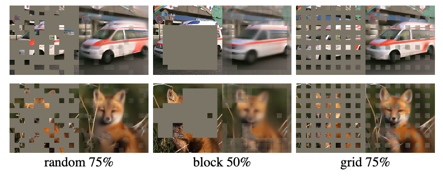
- 저자들은 여러방법을 실험한 끝에 uniform distribution에 따라 mask random sampling을 선택했다.
- block-wise masking방법은 75% 마스킹에서 성능이 낮아지고 대체적으로 blurry한 결과를 보였고 grid-wise방법은 낮은 training loss를 보였지만 representation quality가 낮았다고 한다. (테이블(f) 참고)
Training schedule
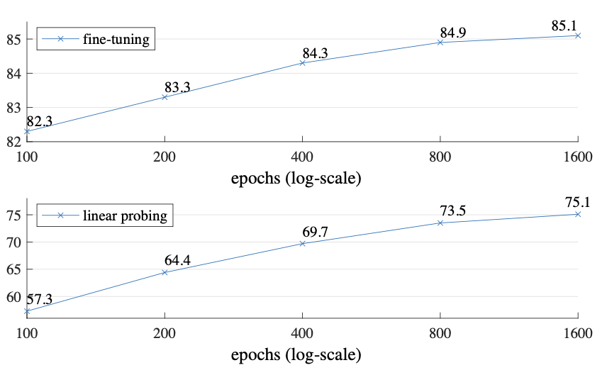
- MAE는 800-epoch pre-training 을 사용하였지만 논문에서는 1600-epoch까지 실험했다.
- ViT-L을 사용한 MoCo v3는 300-epoch에서 saturate되었지만 MAE는 위 그래프에서 볼 수 있듯이 1600epoch을 진행하는 동안에도 아직 saturation되지 않았으며 더 학습할 수 있다는 여지를 남겨 두고 있다.
4.2. Comparisons with Previous Results
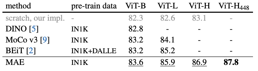
Comparisons with self-supervised methods
- 최근 발표된 Vision분야의 self-supervised 모델과 MAE를 비교하고 있다. ViT-B와 같이 작은 모델은 성능 차이가 크게 나지 않지만 모델이 커질수록 MAE의 강점이 드러난다. 위 표를 보면 알 수 있듯이 MAE는 쉽게 scale up가능하다는 것을 예상할 수 있다.
- 특히 BEiT의 dVAE pre-training 방법을 언급하면서 또 한번의 pre-training을 하지 않아도 충분히 좋은 성능과 함께 simple과 faster가 따라오기 때문에 dVAE pre-training을 MAE에 적용하는 것은 고려하지 않았다고 한다.
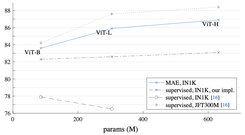
Comparisons with supervised pre-training
- 위 그래프에서 보이는 것처럼 IN1K 데이터셋에서 기존 ViT-L은 ViT-B보다 성능이 더 떨어지지만 MAE 저자들이 implemet하여서 82% 까지 올렸고 MAE는 훨씬 더 많이 올린 것을 볼 수 있다.(파란색)
- 여기서 저자들은 기존 VIT의 JFT300M 데이터셋에 대한 결과의 경향이 MAE의 IN1K 데이터셋에 대한 경향과 비슷하다는 것을 언급하면서 다시한번 MAE의 model size를 scale up 가능하다는 것을 보여주고 있다.
4.3. Partial Fine-tuning
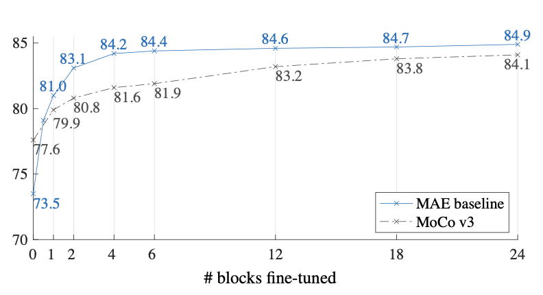
- 위에서 테이블(a~f)을 통해 fine tuning과 linear probing의 차이를 보였다. fine tuning의 성능이 훨씬 좋았고 이 둘의 경향성 또한 달랐다.
- 사실 위에서 보여준 fine tuning의 performance는 end-to-end 즉 모든 block에 대해 fine tuning했을 때의 결과이고 이번에 저자들은 partial tuning에 대해 이야기 하고 있다.
- 지난 몇년동안 linear probing은 인기있는 protocol 이었지만 딥러닝의 강력한 장점인 비선형성을 유지하지 못하는 방법이다.
- 위 그래프에서 보다시피 한개의 transformer block만 fine tuning 하더라도 73.5%에서 81.0%로 정확도가 크게 뛰게 된다는 것을 실험을 통해 보여주고 심지어 절반 block(transformer의 MLP layer 이하)만으로도 엄청난 성능 점핑(79.1%)을 보여준다.
- 즉 backbone을 전부 freeze시키는 것 보다 4~6개의 transformer block을 fine tuning하면 더 좋은 performance를 얻어 낼 수 있다는 것을 저자들은 말하고 있다.
5. Discussion and Conclusion
확장성과 간단함은 딥러닝의 핵심 target이다. NLP에서는 GPT, BERT와 같은 모델이 나오면서 이러한 방향으로 나아가고 있지만 Vision 분야는 self-supervised learning이 고전하고 있지만 supervised learning쪽으로 dominant하다.
이 논문에서는 NLP의 Transformer를 활용하여 Vision의 self-supervised learning분야로 확장 가능성을 제시하였다. 하지만 분명 이미지와 언어는 다른 성격을 지닌 signal이기 때문에 차이를 두고 주의 깊게 다룰 필요가 있다는 것을 강조한다.
Pytorch Implementation
1. Define encoder
import torch
from torch import nn
from einops import rearrange, repeat
from einops.layers.torch import Rearrange

def pair(t):
    return t if isinstance(t, tuple) else (t, t)


# Attention, MLP 이전에 수행되는 Layer Normalization
class PreNorm(nn.Module):
    def __init__(self, dim, fn):
        super(PreNorm, self).__init__()
        self.norm = nn.LayerNorm(dim)
        self.fn = fn

    def forward(self, x, **kwargs):
        return self.fn(self.norm(x), **kwargs)


# 각 쿼리(패치)가 다른 패치와 어느정도 연관성을 가지는지 구하는것이 바로 attention의 목적.
class Attention(nn.Module):
    def __init__(self, dim, heads=8, dim_head=64, dropout=0.):
        super(Attention, self).__init__()
        inner_dim = dim_head * heads  # 512
        project_out = not (heads == 1 and dim_head == dim)

        self.heads = heads  # multi head attention (시퀀스를 병렬로 분할함으로써 다르게 주의를 기울이고 다양한 특징을 얻을 수 있다고 함)
        self.scale = dim_head ** -0.5  # 큰값을 softmax에 올리면 gradient vanishing이 일어나기 때문에 downscale에 사용될 값 (softmax 함수 그래프를 보면 이해가능)

        self.attend = nn.Softmax(dim=-1)
        self.to_qkv = nn.Linear(dim, inner_dim * 3, bias=False)  # query, key, value로 분할하기 위해 3을 곱해줌

        self.to_out = nn.Sequential(
            nn.Linear(inner_dim, dim),
            nn.Dropout(dropout),
        ) if project_out else nn.Identity()

    def forward(self, x):
        qkv = self.to_qkv(x).chunk(3, dim=-1)  # embed dim 기준으로 3분할 (튜플로 감싸져 있음)
        q, k, v = map(lambda t: rearrange(t, 'b n (h d) -> b h n d', h=self.heads), qkv)  # q = k = v (b, heads, num_patches, dim)

        dots = torch.matmul(q, k.transpose(-1, -2)) * self.scale  # query와 key간의 dot product를 위한 차원변경 + scaling
        # dots = (b, heads, num_patches, dim) * (b, heads, dim, num_patches) = (b, heads, num_patches, num_patches)

        attn = self.attend(dots)  # self attention (각 패치간의 연관성을 softmax 확률값으로 나타냄)

        out = torch.matmul(attn, v)  # 구한 확률값을 실제 값(value)에 dot product 시킴 (원래 차원으로 복구) (b, heads, num_patches, dim)
        # out = (b, heads, num_patches, num_patches) * (b, heads, num_patches, dim) = (b, heads, num_patches, dim)
        out = rearrange(out, 'b h n d -> b n (h d)')

        return self.to_out(out)  # 원래 dim으로 복귀


class FeedForward(nn.Module):
    def __init__(self, dim, hidden_dim, dropout=0.):
        super(FeedForward, self).__init__()
        self.net = nn.Sequential(
            nn.Linear(dim, hidden_dim),
            nn.GELU(),
            nn.Dropout(dropout),
            nn.Linear(hidden_dim, dim),
            nn.Dropout(dropout),
        )

    def forward(self, x):
        return self.net(x)


class Transformer(nn.Module):
    def __init__(self, dim, depth, heads, dim_head, mlp_dim, dropout=0.):
        super().__init__()
        self.layers = nn.ModuleList([])
        for _ in range(depth):
            self.layers.append(nn.ModuleList([
                PreNorm(dim, Attention(dim, heads=heads, dim_head=dim_head, dropout=dropout)),
                PreNorm(dim, FeedForward(dim, mlp_dim, dropout=dropout))
            ]))
    def forward(self, x):
        for attn, ff in self.layers:
            x = attn(x) + x  # skip connection
            x = ff(x) + x
        return x


class ViT(nn.Module):
    def __init__(self, *, image_size, patch_size, num_classes, dim, depth, heads, mlp_dim, pool='cls', channels=3, dim_head=64, dropout=0.,
                 emb_dropout=0.):
        super(ViT, self).__init__()
        image_height, image_width = pair(image_size)
        patch_height, patch_width = pair(patch_size)

        assert image_height % patch_height == 0 and image_width % patch_width == 0, '이미지 사이즈를 패치 사이즈로 나눌 수 없음 (Must be divisible)'

        num_patches = (image_height // patch_height) * (image_width // patch_width)  # 이미지의 패치 수
        patch_dim = channels * patch_height * patch_width
        assert pool in {'cls', 'mean'}, 'pool type must be either cls (cls token) or mean (mean pooling)'

        self.to_patch_embedding = nn.Sequential(
            Rearrange('b c (h p1) (w p2) -> b (h w) (p1 p2 c)', p1=patch_height, p2=patch_width),
            nn.Linear(patch_dim, dim),
        )

        self.cls_token = nn.Parameter(torch.randn(1, 1, dim))
        self.pos_embedding = nn.Parameter(torch.randn(1, num_patches + 1, dim))  # class token이 패치 순서 첫번째에 추가되니까 1을 더해줌
        self.dropout = nn.Dropout(emb_dropout)

        self.transformer = Transformer(dim, depth, heads, dim_head, mlp_dim, dropout)

        self.pool = pool
        self.to_latent = nn.Identity()

        self.mlp_head = nn.Sequential(
            nn.LayerNorm(dim),
            nn.Linear(dim, num_classes)
        )

    def forward(self, img):
        x = self.to_patch_embedding(img)  # Rearrange (b, num_patches, patch_dim) -> Linear (b, num_patches, dim)
        b, n, _ = x.shape

        cls_tokens = repeat(self.cls_token, '() n d -> b n d', b=b)  # 각 이미지(배치) 마다 클래스 토큰 보유
        x = torch.cat((cls_tokens, x), dim=1)  # 클래스 토큰이 첫번째로 오도록 하고 패치개수의 차원 dim=1로 concat 시킨다.
        x += self.pos_embedding
        x = self.dropout(x)

        x = self.transformer(x)

        x = x.mean(dim=1) if self.pool == 'mean' else x[:, 0]  # mean은 classification을 전체 패치의 평균값을 사용한다는 것이고 cls는 class token의 값만 사용한다는 것.
        # 논문은 class token이 이미지 전체의 embedding을 표현하고 있음을 가정하기 때문에 class token만 사용하였음.
        x = self.to_latent(x)  # make more compact
        return self.mlp_head(x)  # classification
2. Define MAE
import torch
from torch import nn
import torch.nn.functional as F
from einops import repeat

from vit import Transformer


class MAE(nn.Module):
    def __init__(self, *, encoder, decoder_dim, masking_ratio=0.75, decoder_depth=1, decoder_heads=8, decoder_dim_head=64):
        super(MAE, self).__init__()
        assert masking_ratio > 0 and masking_ratio < 1, 'masking ratio must be kept between 0 and 1'
        self.masking_ratio = masking_ratio

        # some encoder parameters extract
        self.encoder = encoder  # vit encoder
        num_patches, encoder_dim = encoder.pos_embedding.shape[-2:]
        self.to_patch, self.patch_to_emb = encoder.to_patch_embedding[:2]
        pixel_values_per_patch = self.patch_to_emb.weight.shape[-1]  # patch_size * patch_size * 3 (패치당 픽셀 개수(rgb))
        # decoder parameters
        self.enc_to_dec = nn.Linear(encoder_dim, decoder_dim) if encoder_dim != decoder_dim else nn.Identity()
        self.mask_token = nn.Parameter(torch.randn(decoder_dim))
        self.decoder = Transformer(dim=decoder_dim, depth=decoder_depth, heads=decoder_heads, dim_head=decoder_dim_head, mlp_dim=decoder_dim*4)
        self.decoder_pos_emb = nn.Embedding(num_patches, decoder_dim)
        self.to_pixels = nn.Linear(decoder_dim, pixel_values_per_patch)

    def forward(self, img):
        device = img.device

        # get patches
        patches = self.to_patch(img)
        batch, num_patches, *_ = patches.shape  # (b, 64, 3072)  not in class token

        tokens = self.patch_to_emb(patches)  # shape (b, 64, 1024)
        tokens = tokens + self.encoder.pos_embedding[:, 1:(num_patches+1)]  # not in class token

        # mask, unmask의 랜덤인덱스를 생성
        num_masked = int(num_patches * self.masking_ratio)  # int(64 * 0.75) = 48
        rand_indices = torch.rand(batch, num_patches, device=device).argsort(dim=-1)  # 배치별로 패치에 uniform distribution으로 랜덤 index 부여(논문에서 uniform distribution 사용)
        masked_indices, unmasked_indices = rand_indices[:, :num_masked], rand_indices[:, num_masked:]  # shape (b, 48) (b, 16)

        # unmasked 위치의 토큰값만 인덱싱
        batch_range = torch.arange(batch, device=device)[:, None]  # shape (b, 1)
        tokens = tokens[batch_range, unmasked_indices]  # 마스크가 아닌 위치의 embed값만 인덱싱함  shape (b, 16, 1024)

        # reconstruction loss를 계산하기 위한 정답 masked_patches
        masked_patches = patches[batch_range, masked_indices]  # shape (b, 48, 3072)

        # encoding
        encoded_tokens = self.encoder.transformer(tokens)

        # project encoder to decoder dimensions, if they are not equal - the paper says you can get away with a smaller dimension for decoder
        decoder_tokens = self.enc_to_dec(encoded_tokens)

        # repeat mask token
        mask_tokens = repeat(self.mask_token, 'd -> b n d', b=batch, n=num_masked)  # (b 48 512)
        mask_tokens = mask_tokens + self.decoder_pos_emb(masked_indices)  # mask_token도 positional embedding 추가

        # concat tokens and decoding
        # position embedding을 둘다 주었기 때문에 원래 sequence로 돌려놓지 않고 바로 concat시킴
        decoder_tokens = torch.cat((mask_tokens, decoder_tokens), dim=1)  # shape (b, 64, 512)
        decoded_tokens = self.decoder(decoder_tokens)

        mask_tokens = decoded_tokens[:, :num_masked]  # 위에서 concat을 mask먼저 했으므로 이렇게 mask 정보만 인덱싱
        pred_pixel_values = self.to_pixels(mask_tokens)  # (b, 48, 3072)

        # calculate reconstruction loss

        recon_loss = F.mse_loss(pred_pixel_values, masked_patches)
        return recon_loss
3. Test
import torch
from vit import ViT
from mae import MAE
import timm

if __name__ == '__main__':
    v = ViT(
        image_size=256,
        patch_size=32,
        num_classes=1000,
        dim=1024,
        depth=6,
        heads=8,
        mlp_dim=2048
    )

    mae = MAE(
        encoder=v,
        masking_ratio=0.75,  # the paper recommended 75% masked patches
        decoder_dim=512,  # paper showed good results with just 512
        decoder_depth=6  # anywhere from 1 to 8
    )

    images = torch.randn(8, 3, 256, 256)

    loss = mae(images)
    print(f"Masked Autoencoders MSE Loss: {loss:.5f}")
output :
Masked Autoencoders MSE Loss: 1.83466
End
이번 논문을 통해 이제는 정말 task간의 장벽이 허물어지고 다른 task의 방법론을 자신의 task에 적용하는 방식의 연구가 많이 이루어지고 있다는 것을 느꼈다.
요즘 많은 딥러닝 사용자들이 겪고 있는 라벨링 문제를 벗어날 수 있는 Self-Supervised Learning이 Vision분야에서 더 활발해져서 GPT, BERT와 같이 Vision에서도 대표적인 모델이 하나 생겼으면 하는 바램이다.
Keep going
Reference
- Paper - https://arxiv.org/abs/2111.06377
- Review1 - https://youtu.be/mtUa3AAxPNQ
- Review2 - https://youtu.be/LKixq2S2Pz8
Leave a comment